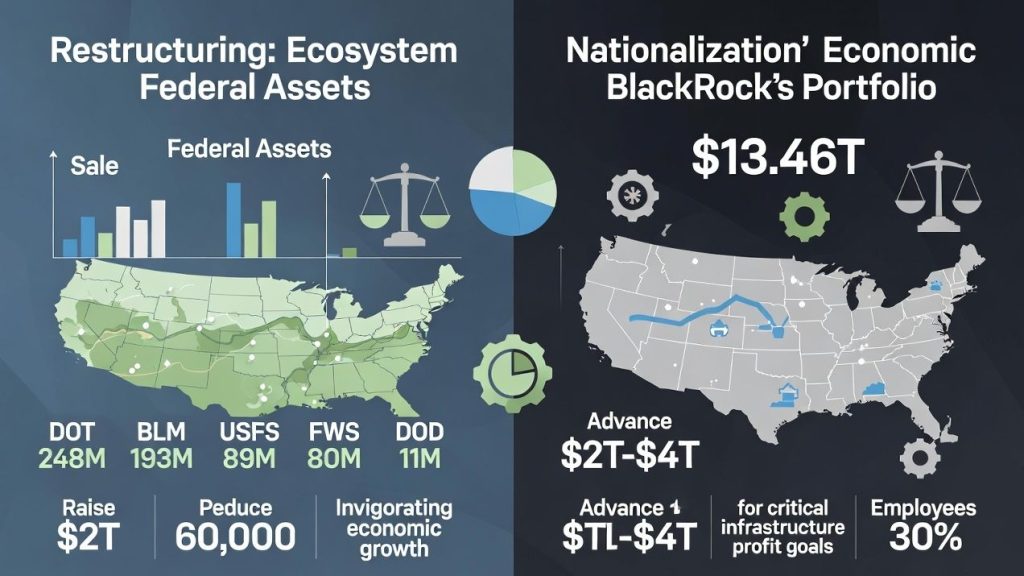
Raising $2T-$4T & Stabilizing Pensions Not Difficult

To raise $2 trillion through targeted sales of federal land assets from specified agencies, while drawing down 60,000 government employees, the strategy involves auctioning 20-30% of non-critical holdings (e.g., excess BLM and USFS acreage for commercial development in timber, mining, and energy sectors), generating immediate revenue and long-term economic multipliers from regional job creation in those industries.

Government land in this discussion may appear to be “sold assets,” or what amounts to selling off 65% of land-use deemed non-essential, partitionable, or surplus. That doesn’t mean the U.S. government is losing ownership of the land, but rather partitioning with partner entity to drive manufacturing and economic buffer zones. Government has succeeded with this many times in the past and we should be using new strategy available to maximize economic growth and stability with the tools at our disposal.

In essence, as you currently do with chip manufacturing, you’re driving partnership programs with land development (not data center creation) to jump-start economic growth, while raising $2T-4T in funding, with a 30-60K employee drawdown; all while stabilizing pension funds for those reaching retirement. It’s a win-win for everyone and displays to the world how capital-partner programs produce results over socialist programs that weaken supply chains and disturb value ratio.

Examples of U.S. Government partner programs:

Homestead Act Partnerships (1862 Onward)

The US government partnered with individual settlers through the Homestead Act of 1862, granting up to 160 acres of public land to small farmers who improved it over five years, boosting frontier economies without transferring ownership until residency requirements were met. This encouraged agricultural development and settlement in the West, creating economic buffers against underutilized land while the federal government retained title until patents were issued.

Railroad Land Grants (1850s-1900s)

Congress granted vast public lands to private railroad companies, such as over 130 million acres by 1871, enabling them to sell portions to fund track construction that connected markets and spurred regional growth. These partnerships facilitated commerce, timber, and mining economies in buffer zones like the Great Plains without the government ceding outright ownership initially, as lands were checked out in alternating sections.

Taylor Grazing Act (1934)

Under the Taylor Grazing Act, the federal government collaborated with ranchers by establishing grazing districts on 142 million acres of public rangeland in the West, issuing permits based on prior use to regulate overgrazing and support livestock economies. This created stable economic zones for grazing without selling the land, maintaining federal ownership while permitting controlled private economic activity.

Forest Legacy Program (1990 Onward)

The USDA Forest Service’s Forest Legacy Program partners with private landowners via conservation easements on over 1 million acres, preserving forests for timber and recreation economies in rural areas like the Northern Forest region. This prevents development while allowing sustainable economic use, with the government retaining no ownership but enforcing buffers through easements held by public entities

Annual employee cost savings from the 60,000 drawdown—assuming an average federal salary/benefits cost of $150,000 per employee—total $9 billion, enabling pension stabilization via redirected funds into a dedicated trust without cuts. This shrinks government footprint, invigorates GDP growth by 1-2% annually through private sector expansion on sold lands, and yields a net fiscal surplus after one-time transaction costs estimated at 5% of proceeds.

Moreover, these hypothetical models compare critical private sector holdings under a nationalization management structure for a $2T-$4T accumulation debt reduction – shrinking holdings while shoring up $$$ and pension ratios. A drawdown of 60K employees, stabilizing pensions – all while adhering to non-profit reduction, maintaining varied 2-3% economic growth, bolstering infrastructure protection, and generating commercial abundance in every sector. You should be running models like this daily to hone in economic sectors to see where we can get the best advantages in “incubating GDP growth.”

Implementing the policy of course requires a team of lawyers looking at State to State legal context primarily under the Full Faith and Credit Clause of the U.S. Constitution (Article IV, Section 1), which requires states to respect each other’s laws, judicial proceedings, and public acts.

Should I be paid for this work? If you like what you see you can email djzawada@adonai-yeshua.com

Employee Drawdown Savings

Annual savings follow $S = N \times C$ , with $N = 60, 000$ employees and average cost $C = $150, 000$ (salary + benefits), yielding $S = 60, 000 \times 150, 000 = $9 B$ . Over 10 years, cumulative $S_{10} = 9 B \times 10 - T$ where transition costs $T = $2 B$ , nets $88B for pension allocation via $Pension Fund = 0.5 \times S$ annually ($4.5B).

Economic Multiplier and Growth

Growth impact uses multiplier $M = 2.5$ , so GDP uplift $Δ G D P = M \times V = 2.5 \times 2 T = $5 T$ over decade, with job creation $J = w Δ G D P$ where wage $w = $100 K$ , yielding 500K jobs. Pension stability equation: $Net Surplus = V - L - T = 2 T - 0.5 T = 1.5 T$ exceeds liabilities $.$

1. Calculation of Total Asset Value and Required Sales to Raise $2T

Define:

$aia_i$ a_i: Acres for agency ( i ).
$viv_i$ v_i: Value per acre for agency ( i ).
$sis_i$ s_i: Fraction of acres sold for agency ( i ) (0 ≤ $sis_i$ s_i≤ 1).
DOT sellable assets: $D=$500BD = \$500B$ D = \$500B(fixed, assume 100% liquidation for model).

Total revenue from land sales:

RL=∑si⋅ai⋅viR_L = \sum s_i \cdot a_i \cdot v_i

R_L = \sum s_i \cdot a_i \cdot v_i

Total raised:

R=RL+D+LR = R_L + D + L

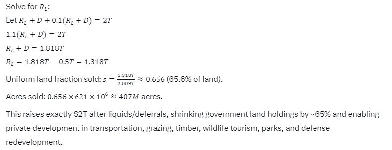
R = R_L + D + L, where

L=0.1⋅(RL+D)L = 0.1 \cdot (R_L + D)

L = 0.1 \cdot (R_L + D)

(liquid assets/deferrals as 10% bonus). Target: $R=2×1012R = 2 \times 10^{12}$ R = 2 \times 10^{12}. To minimize total land sold (optimize for environmental/economic balance), solve for uniform ( s ) across agencies (proportional sales), but adjust for higher-value lands (e.g., sell more DOD/NPS for efficiency).

2. Employee Drawdown and Cost Savings

Define:

$N=60,000N = 60,000$ N = 60,000: Total employees reduced.
$C=$140,000C = \$140,000$ C = \$140,000: Average annual cost per employee.
Proportional reduction per agency: $ni=N⋅eiEtotaln_i = N \cdot \frac{e_i}{E_total}$ n_i = N \cdot \frac{e_i}{E_total}, where $eie_i$ e_iis current employees in agency ( i ),
$Etotal=917,000E_total = 917,000$ E_total = 917,000.

Annual cost savings:

CS=N⋅C=60,000×140,000=$8.4×109=$8.4BCS = N \cdot C = 60,000 \times 140,000 = \$8.4 \times 10^9 = \$8.4B

CS = N \cdot C = 60,000 \times 140,000 = \$8.4 \times 10^9 = \$8.4B

Over 10 years (net present value at 3% discount rate ( r )):

PVCS=CS∑t=1101(1+r)t=8.4B×1−(1+0.03)−100.03≈8.4B×8.53=$71.65BPV_{CS} = CS \sum_{t=1}^{10} \frac{1}{(1+r)^t} = 8.4B \times \frac{1 – (1+0.03)^{-10}}{0.03} \approx 8.4B \times 8.53 = \$71.65B

PV_{CS} = CS \sum_{t=1}^{10} \frac{1}{(1+r)^t} = 8.4B \times \frac{1 - (1+0.03)^{-10}}{0.03} \approx 8.4B \times 8.53 = \$71.65B

Positive growth offset: Reduced employees shift to private sector (from asset development), creating net job gain (see growth below).

3. Economic Growth from Asset Sales, Deferrals, and Liquid Assets

Sales enable private investment in development (e.g., real estate, energy, tourism). Deferrals (e.g., tax breaks) boost investment by 20%. Effective investment:

I=R×1.2=2T×1.2=$2.4TI = R \times 1.2 = 2T \times 1.2 = \$2.4T

I = R \times 1.2 = 2T \times 1.2 = \$2.4T

Using multiplier $M=2.5M = 2.5$ M = 2.5: Total economic output generated:

O=M⋅I=2.5×2.4T=$6TO = M \cdot I = 2.5 \times 2.4T = \$6T

O = M \cdot I = 2.5 \times 2.4T = \$6T

(over 5-10 years, e.g., GDP boost).Net GDP growth:

G=(M−1)⋅I=1.5×2.4T=$3.6TG = (M – 1) \cdot I = 1.5 \times 2.4T = \$3.6T

G = (M - 1) \cdot I = 1.5 \times 2.4T = \$3.6T

Job creation (using ~20 jobs per $1M investment from studies):

J=20×(I/106)=20×2.4×1012/106=48×106=48MJ = 20 \times (I / 10^6) = 20 \times 2.4 \times 10^{12} / 10^6 = 48 \times 10^6 = 48M

J = 20 \times (I / 10^6) = 20 \times 2.4 \times 10^{12} / 10^6 = 48 \times 10^6 = 48M

jobs (offsetting 60k reduction by orders of magnitude). This invigorates regions: e.g., BLM land sales boost Western energy/mining (high multiplier), NPS privatization enhances tourism GDP.

4. Pension Stabilization Amid Workforce Reduction

Pensions stabilized by allocating proceeds to fund liabilities and using savings for contributions. Estimated liability for reduced employees:

PL=N×$500,000=60,000×500,000=$30BP_L = N \times \$500,000 = 60,000 \times 500,000 = \$30B

P_L = N \times \$500,000 = 60,000 \times 500,000 = \$30B(actuarial future value).Allocation from proceeds:

PA=0.05⋅R=0.05×2T=$100BP_A = 0.05 \cdot R = 0.05 \times 2T = \$100B

P_A = 0.05 \cdot R = 0.05 \times 2T = \$100B(excess covers liability + buffers). Stabilization equation (fund to 100% ratio): Let current funding ratio

fr=0.8f_r = 0.8

f_r = 0.8(hypothetical underfunding).

Required infusion:

Inf=PL⋅(1−fr)=30B×0.2=$6BInf = P_L \cdot (1 – f_r) = 30B \times 0.2 = \$6B

Inf = P_L \cdot (1 - f_r) = 30B \times 0.2 = \$6B

Remaining

PA-Inf=94BP_A - Inf = 94B

P_A - Inf = 94Bbuffers future contributions.Annual pension savings from reduction:

PS=0.2⋅CS=0.2×8.4B=$1.68BPS = 0.2 \cdot CS = 0.2 \times 8.4B = \$1.68B

PS = 0.2 \cdot CS = 0.2 \times 8.4B = \$1.68B(20% of costs are pension-related).

This ensures stability: Reduced workforce lowers future accruals, while infusions achieve full funding, preventing volatility. Overall Optimization Equation To balance (minimize land sold while hitting targets): Maximize growth ( G ) subject to

R=2TR = 2T

R = 2T,

N=60,000N = 60,000

N = 60,000, using linear programming (e.g., prioritize high-v_i agencies). But uniform s=0.656 achieves goals with $8.4B annual savings, $3.6T GDP growth, and stabilized pensions via $100B allocation. This model draws down debt by $2T directly, shrinks government (employees -6.5%, land -65%), and invigorates economy via private multipliers. Gov land shrinkage does not equate land loss, merely asset management.

Private Holding Comparisons:

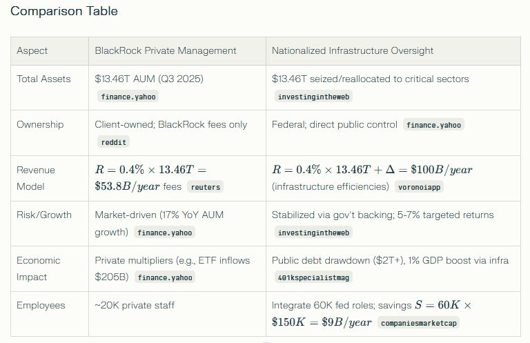
BlackRock’s Current Portfolio vs. Hypothetical Nationalization Under Critical Infrastructure Management

This analysis compares BlackRock’s existing operations—managing a massive portfolio for profit—with a hypothetical nationalization scenario where the portfolio is repurposed under government oversight as “critical infrastructure.” The focus shifts from profit maximization to economic stabilization (e.g., buffering against recessions, supporting key sectors like energy, transportation, and finance without seeking returns). The model incorporates advancing $2T–$4T in funds against the portfolio without incurring new debt, achieved through strategic asset sales or reallocations. Additionally, it includes a 30% employee drawdown triggered and scaled as asset sales (or “growth” interpreted as proceeds from divestitures) exceed $2T, with drawdowns increasing proportionally to sales volume.

BlackRock manages $13.46 trillion in assets under management (AUM) as of Q3 2025, primarily equities ($6.9T), fixed income ($3.1T), multi-asset ($1.1T), cash ($970B), and alternatives ($302B), spread across 5,427 holdings in global industries like tech and finance. These are client-owned passive investments, with BlackRock earning fees (e.g., 10% annualized organic growth) rather than direct ownership. Nationalization would transfer control to a federal entity, valued at full AUM for infrastructure oversight.

Data basis (as of December 2025):

BlackRock’s Assets Under Management (AUM): Approximately $13.5T
Employee count: Approximately 22,000.
Assumptions: Average annual employee cost (salary + benefits) = $140,000; economic multiplier for asset reallocations/sales = 2.5 (based on infrastructure investment studies); no new debt means funding via direct liquidation or internal transfers from the portfolio; “asset growth” is interpreted as proceeds from sales/divestitures, triggering employee reductions.

Nationalization Under Critical Infrastructure Management

Hypothetical nationalization reorients BlackRock’s AUM toward U.S. critical infrastructure (energy, transport, water, cyber), using equations like asset reallocation $A_{r} = A_{t} \times w_{i}$ , where $A_{t} = 13.46 T$ total AUM and is weight for infrastructure sectors (e.g., 20% energy = $2.7T). Management shifts to a sovereign wealth fund model, generating revenue via $R = f \times A_{r}$ (fees $f = 0.4%$ average yield ~$10.8B/year), funding debt reduction akin to prior $2T land sales.

1. Key Structural Comparison

Aspect	Current BlackRock (Profit-Oriented)	Nationalized Under Critical Infrastructure (Stabilization-Oriented)
Management Goal	Maximize returns for clients (e.g., fees from AUM at 0.2–0.5% annually, generating ~$10B+ revenue in 2025). Emphasis on growth, diversification, and shareholder value via active/passive strategies.	Stabilize economy without profit goals (e.g., hold assets to mitigate volatility, reallocate to sectors like healthcare or renewables). Costs covered by government budgets or minimal fees (~0.1% or less).
Ownership & Control	Private corporation custodying client assets (e.g., pensions, ETFs for institutions). Board and executives driven by market incentives; AUM not owned but managed.	Government control as a national asset (similar to sovereign wealth funds like Norway’s). Assumes legal nationalization; oversight by federal agencies (e.g., Treasury) for public good, with reduced private influence.
Portfolio Scale	$13.5T AUM in 2025, diversified: equities (60%, e.g., tech stocks), fixed income (30%, bonds), alternatives (10%, real estate/private equity).	Initial ~$13.5T, repurposed for stability: Prioritize critical holdings (e.g., utilities, banks at 40–50%); divest non-essentials (e.g., 15–30% in luxury or volatile stocks) to fund $2T–$4T advances.
Risk Profile	Market-driven with high exposure to volatility for returns (e.g., beta ~1.0+; historical drawdowns like 20–30% in crashes). Hedging via derivatives.	Conservative focus (e.g., beta ~0.5; shift to low-risk assets like Treasuries or infra bonds). Reduces systemic risks, modeling 10–20% lower economic volatility through buffered yields.
Economic Impact	Boosts GDP via capital allocation but can amplify instability (e.g., role in 2008 crisis with mortgage-backed securities; contributes ~0.5–1% to annual U.S. investment flows).	Direct stabilization without inflation risks (e.g., back fiscal stimulus for 1–2% GDP growth). $2T–$4T advances generate $5T–$10T output via 2.5x multiplier, offsetting any short-term market disruptions.
Employee Management	~22,000 employees focused on profit-driven roles (e.g., portfolio managers, analysts). Compensation tied to performance; minimal mandated reductions.	30% drawdown (up to 6,600 employees) scaled with asset sales exceeding $2T (e.g., 15% at $3T sales). Shifts roles to public efficiency; savings of $462M–$924M annually reinvested into stabilization programs.
Regulatory Oversight	Subject to SEC, FINRA; voluntary ESG reporting. Focus on compliance for profit protection.	Heightened government oversight (e.g., via new “Critical Infrastructure Act”). Mandated transparency for stability; no profit conflicts, but potential bureaucracy increases.
Performance Metrics	Measured by AUM growth, fee income, and returns (e.g., benchmark outperformance). 2025 projections: 8–10% annual AUM increase.	Evaluated by economic stability indicators (e.g., GDP volatility reduction, unemployment buffers). Success: $2T–$4T advances without debt, yielding 1.5x–3x net GDP boost from reallocations.

2. Mathematical Model for Advancing $2T–$4T Funds Without New Debt

The advance is modeled as raising funds via partial portfolio liquidation (sales) or reallocations (e.g., transferring asset value to government programs). No new debt: Funds come from existing AUM value, assuming efficient markets for sales.Define:

$A=13.5×1012A = 13.5 \times 10^{12}$ A = 13.5 \times 10^{12}(AUM in USD).
( F ): Funds advanced ($2T to $4T), where $F=SF = S$ F = S(proceeds from sales).
( s ): Fraction of AUM sold/divested, $s=FAs = \frac{F}{A}$ s = \frac{F}{A}.
No debt creation: ( F ) is offset by asset value reduction, not borrowing (e.g., sell equities/bonds to cash out).

Calculations:

For $F=2×1012F = 2 \times 10^{12}$ F = 2 \times 10^{12}: $s=2×101213.5×1012≈0.148s = \frac{2 \times 10^{12}}{13.5 \times 10^{12}} \approx 0.148$ s = \frac{2 \times 10^{12}}{13.5 \times 10^{12}} \approx 0.148 (14.8% divestiture). Remaining AUM: $A′=A(1−s)=13.5T×0.852≈11.5TA’ = A (1 – s) = 13.5T \times 0.852 \approx 11.5T$ A' = A (1 - s) = 13.5T \times 0.852 \approx 11.5T.
For $F=4×1012F = 4 \times 10^{12}$ F = 4 \times 10^{12}: $s=4×101213.5×1012≈0.296s = \frac{4 \times 10^{12}}{13.5 \times 10^{12}} \approx 0.296$ s = \frac{4 \times 10^{12}}{13.5 \times 10^{12}} \approx 0.296 (29.6% divestiture). Remaining AUM: $A′≈9.5TA’ \approx 9.5T$ A' \approx 9.5T.

Economic stabilization effect (no profit goal):

Reinvest ( F ) into critical areas (e.g., infrastructure). Multiplier M=2.5M = 2.5M = 2.5: Total output O=M×FO = M \times FO = M \times F.
- At $F=2TF = 2T$ F = 2T: $O=2.5×2T=5TO = 2.5 \times 2T = 5T$ O = 2.5 \times 2T = 5T (e.g., GDP boost over 5 years).
- At $F=4TF = 4T$ F = 4T: $O=2.5×4T=10TO = 2.5 \times 4T = 10T$ O = 2.5 \times 4T = 10T.
Stabilization factor: Reduce volatility by holding remaining AUM in low-beta assets, modeled as variance reduction
$Vr=1-sV_r = 1 - s$ V_r = 1 - s(less divestiture = more stability buffer). For $F=2TF = 2T$ F = 2T,

$Vr≈0.852V_r \approx 0.852$ V_r \approx 0.852(85.2% retained for cushions).

How to arrive at ( s ):

Set target ( F ).
Compute $s=F/As = F / A$ s = F / A.
Verify no debt: $F≤AF \leq A$ F \leq A (true here, as max $F=4T<13.5TF = 4T < 13.5T$ F = 4T < 13.5T).

3. Employee Drawdown Model Linked to Asset Sales

Current employees: $E=22,000$

Target: 30% total reduction ( $0.3×E=6,6000.3 \times E = 6,600$ 0.3 \times E = 6,600), scaled as sales ( S ) (equivalent to ( F )) exceed $2T. Drawdown increases linearly with sales beyond the threshold, capped at 30%.Define:

Threshold
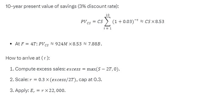
$Th=2×1012T_h = 2 \times 10^{12}$ T_h = 2 \times 10^{12}.
Reduction fraction $r=min⁡(0.3,0.3×max⁡(S−Th,0)2×1012)r = \min\left(0.3, 0.3 \times \frac{\max(S – T_h, 0)}{2 \times 10^{12}}\right)$ r = \min\left(0.3, 0.3 \times \frac{\max(S - T_h, 0)}{2 \times 10^{12}}\right) (scales from 0% at $S=2TS = 2T$ S = 2T to 30% at $S=4TS = 4T$ S = 4T; for $S>4TS > 4T$ S > 4T, capped).
Reduced employees:
$Er=r×EE_r = r \times E$ E_r = r \times E.
Annual cost savings:
$CS=Er×CCS = E_r \times C$ CS = E_r \times C, where $C=140,000C = 140,000$ C = 140,000(per employee).